“The first rule of investing is never lose money” – Warren Buffett
Interest in investing seems to be at an all-time high right now. People of all ages and wealth statuses are looking to invest in numerous asset classes across both public and private markets.
This is wonderful. More people interested in investing should hopefully result in more people achieving financial security.
To achieve that goal, investors need to leverage the most powerful force available to them, compounding. However, most people focus on arithmetic returns when making investment decisions, which puts the goal at risk. Analyzing investments based on arithmetic returns creates a higher chance of losing money. What successful investors do is evaluate investment opportunities through the lens of geometric returns.
That is exactly what we will dive into in this essay: What are geometric and arithmetic returns? Why does focusing on geometric returns lead to better decision-making? How can you use this concept to make smarter bets?
Having The Right Perspective
When evaluating investments, we can adopt either an arithmetic or a geometric view. The perspective we choose will determine which opportunities we pursue.
An arithmetic return is the average we are all familiar with. It is the sum of a series of returns, divided by the total amount of series. This is the simple average most people are familiar with and the most common way to evaluate opportunities.

Geometric averages are calculated differently. Multiply all the returns (plus 1) and raise it to the inverse of the length of the series.

Understanding the formulas is not important. What is essential is to remember that we should examine investment returns through a geometric lens because doing so accounts for compounding.
Why am I placing such emphasis on compounding?
Investing is a process that happens sequentially through time. It does not occur in just one interval of time, or the aggregate of many intervals of time. This means that returns are an iterative process; returns compound. In each period we invest what we are left with from the last period. Thus, the starting size of our capital base will determine how large our compound interest will be.
This is the principle that fundamentally determines the nature of investing and the way we need to interpret returns. Looking at geometric returns is how we capture this principle in metrics.
As critical as this concept is, the difference between these two metrics is not intuitive. To make it more tangible, let’s look at a gambling example.
Playing Dice
Imagine you are at a casino table with a big stack of cash in front of you—your entire life savings of $100. You are going to play a game of dice.
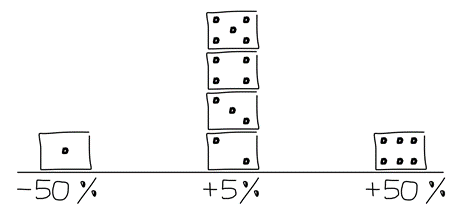
The rules are as follows:
- If you roll a 1, you lose 50% of your entire savings
- If you roll a 2, 3, 4, or 5, you make 5% of your entire savings
- If you roll a 6, you make 50% of your entire savings
- You can play as many times as you want
Would you play?
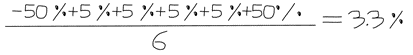
The proposition sounds like a symmetrical bet with an obvious edge from the extra 5% you should get 2/3rds of the time. The expected arithmetic return is 3.3%.
Now, you might have some hesitation if you were allowed to play the game once and you rolled a 1. Playing once exposes you to being unlucky and having your wealth cut in half. Playing numerous times should remove luck from the equation and result in an average expected return of 3.3%. So, you decide to play.
What would your outcome be?
Using a Monte Carlo simulation, the table below shows your chances of ending up in different wealth buckets assuming you play the game 300 times.
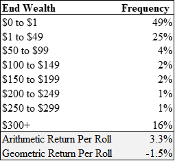
Playing this game results in a ~50% chance of ending up with less than $1 and a ~80% chance of having less than your initial $100. Yet, the arithmetic expected return is 3.3%.
What gives?
The culprit is how arithmetic averages are calculated.
The simulation resulted in many outcomes with low ending wealth values but a few outcomes with incredibly high ending wealth values. The high but unlikely outcomes are so good that they lift up the arithmetic average.
Here’s another way of thinking about this: If Bill Gates walks into a bar with nine people, on average there will be 10 billionaires at the bar.
This should highlight the difference between the most likely outcome and the average outcome. As investors, we should focus on the most likely outcome to avoid the arithmetic trap. This is where geometric returns come in.
When we consider the geometric average, it is clear that this is a bad bet. We lose -1.5% of our wealth per roll. Compounded over 300 rolls, we are essentially left with nothing.
Math Or Magic?
Based on the above, we might assume that never playing this game is the right answer.
However, that isn’t quite true. When you focus on increasing geometric returns, magical things start to happen.
Let’s keep the same game but add one additional rule: You can choose to bet as much of your wealth as you want.
Based on this new rule, you now bet 40% of your capital base on each roll instead of going all-in. You keep the remaining 60% on the sideline earning nothing.
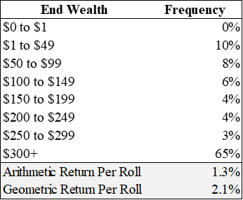
By betting less of your wealth, your arithmetic average falls predictably by 60%—from 3.3% to 1.3%. But before you get disappointed, remember that geometric average is what really counts. When we park money on the sideline, our geometric average increases to 2.1%.
When you play 300 times, you end up making money in ~82% of the outcomes, with an expected ending wealth of ~$700, an increase of ~7x your starting wealth.
Pause there for a second and let that simmer.
We lowered our risk profile by parking 60% of our net worth out of the bet and increased our return.
Doesn’t that violate the risk & return tradeoff—a core pillar of traditional finance? How did we get a higher geometric return by betting less? Is this math or magic?
The answer involves the relationship between two competing forces: (1) the edge of a specific investment or bet and (2) a concept called Negative Geometric Drag (NGD).[1]
The edge of an investment or bet is the mathematical advantage you have. Sticking to the example above, our edge is the 3.3% arithmetic advantage.
NGD is the drag on your return caused by gaining and then losing the same proportion of your wealth. It is based on the principle that a loss disproportionally hurts you because it reduces your capital base for the next investment opportunity. For example, if you have $100 and you lose 50%, your ending wealth is $50. To grow your wealth back to $100, you need more than a 50% return; you need a 100% return since your starting wealth is now $50.

You can think of the relationship between the edge and the NGD as a seesaw.
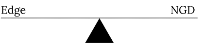
When you bet a lower percentage of your total wealth, the edge is the more powerful force and the NGD is negligible. However, as the portion of the investment size as a percentage of your total wealth increases, the NGD becomes the more powerful force and the impact of a loss hurts you more than the edge. [2] This is because the edge of an investment grows linearly to the amount invested but, NGD grows exponentially. [3]
Protect Your Capital
In all the situations described above, we had certainty over probabilities and outcomes. The real world is not as precise. But there are still useful principles and heuristics we can extract.
The most important is to focus on geometric returns and compounding.
Remember, when we invest, the capital base we start with is the ending capital base from the last period. The capital base is the very thing returns are built on. This means a large loss disproportionately lowers our geometric return because it leaves us with a much lower capital base to reinvest and compound on our next wager.
More tactically, this means taking steps to preserve your capital base. [4] This doesn’t mean avoiding risky bets; rather it requires you to understand how to size your position in risky bets, so your edge is greater than the NGD.
With that, I will leave you with Buffett’s second rule of investing: “Never forget rule number 1.”
Notes, Inspirations & Additional Readings
Thanks to Kerri & Charlotte for their review and feedback.
[1] Nick Yoder explores this concept in more detail in his article “The Kelly Criterion”.
[2] If you want to look at the mathematical logic driving this concept, I have linked a Google sheet here.
[3] The optimal ratio between the NGD and the edge is called the Kelly Criterion, but we won’t dive into that today.
[4] Having this perspective should also fundamentally change how you perceive certain risk management products such as insurance, sitting on cash, or other safe haven assets. You can think of insurance as a drag on your arithmetic return but a boost in your geometric return. When the boost in geometric return is larger than the drag in arithmetic return, it is a good trade. More importantly, insurance can be positive sum, with both the insurer and the insured winning. For more on this, I recommend that you read Safe Haven by Mark Spitznagel.